In[16]:= eqns = 8f''@xd == g@xd, f@xd + g@xd == 3 sin@xd, f@pid == 1, f'@pid == 0<; However we can solve the equation without any initial conditions:

Pin On Calculusdiffyq Hacks
Since a homogeneous equation is easier to solve compares to its

How to solve differential equations with initial conditions. F ( 0) = a f (0)=a f ( 0) = a. This question already has answers here : From scipy.integrate import odeint import numpy as np import matplotlib.pyplot as plt c = 1.0 #value of constants #define function def exam (y, x):
An example of using odeint is with the following differential equation with parameter k=0.3, the initial condition y 0 =5 and the following differential equation. With boundary value problems we will have a differential equation and we will specify the function and/or derivatives at different points, which we’ll call boundary values. Dy dx = g(x) f (y).
For instance, for a second order differential equation the initial conditions are, y(t0) = y0 y′(t0) = y′ 0 y ( t 0) = y 0 y ′ ( t 0) = y 0 ′. Solutions to particular, general, and initial conditions. The syntax is the same as for a system of ordinary differential equations.
For differential equations of the first order one can impose initial conditions in the form of values of unknown functions (at certain points for odes) but on the other hand for certain initial conditions there are no solutions and this is the case we encounter here. X → ( t) = e λ 1 t v → 1 = e t ( − 1 1), x → ( t) = e λ 2 t v → 2 = e − t ( 1 1). With the initial conditions $y(0)=1,y'(0)=0$, the particular solution is $y_c(x):=\cos x$, and with the inital conditions $y(0)=0,y'(0)=1$, $y_s(x):=\sin x$.
{ x 1 ′ ( t) = − x 2 ( t) x 2 ′ ( t) = − x 1 ( t) i have found the linearly independent solutions. This example has shown us that the method of laplace transforms can be used to solve homogeneous differential equations with initial conditions without taking derivatives to solve the. Find solutions for an differential equation system (2 answers) closed 4 years ago.
However, this method only solves the equations for one initial condition at a time. {\displaystyle x=0.} the number of initial conditions required to find a particular solution of a differential equation is also equal to the order of the equation in most cases. I have used the matlab command dsolve
Given a matrix v to be and (w transpose) wt=, find x'= v*x + w by solving the set of linear differential equations with initial conditions to be xi(0)=1 for 1<=i<=7. D 3 u d x 3 = u , u ( 0 ) = 1 , u ′ ( 0 ) = − 1 , u ′ ′ ( 0 ) = π. The next two sections describe techniques to solve for many different initial conditions.
Included are most of the standard topics in 1st and 2nd order differential equations, laplace transforms, systems of differential eqauations, series solutions as well as a brief introduction to boundary value problems, fourier series and partial differntial equations. The model, initial conditions, and time points are defined as inputs to odeint to numerically calculate y(t). For your kind consideration i'm giving below the code that could solve the differential equation:
⇒ f (y) = g(x) + c, where f and g are antiderivatives of f and g, respectively. How you solve them depends on if you need a general or particular solution, or if an initial value problem is specified. Given this additional piece of information, we’ll be able to find a value.
To solve the equations for different initial population sizes, change the values in p0 and rerun the simulation. By integrating both sides, ⇒ ∫f (y)dy = ∫g(x)dx, which gives us the solution expressed implicitly: By multiplying by dx and by f (y) to separate x 's and y 's, ⇒ f (y)dy = g(x)dx.
A differential equation comes in many different guises. Here is a set of notes used by paul dawkins to teach his differential equations course at lamar university. Second order linear homogeneous differential equations with constant coefficients for the most part, we will only learn how to solve second order linear equation with constant coefficients (that is, when p(t) and q(t) are constants).
If we want to find a specific value for c c c, and therefore a specific solution to the linear differential equation, then we’ll need an initial condition, like. In this work, we posit the problem of approximating the solution of a fixed partial differential equation for any arbitrary initial conditions as learning a conditional probability. Y(t)$$ the python code first imports the needed numpy, scipy, and matplotlib packages.
The only way to solve for these constants is with initial conditions. As we chose the canonical basis, the solution for arbitrary initial conditions is $$y(x)=y(0) y_c(x)+y'(0) y_s(x).$$ I want to solve the following differential equation with initial conditions:
Therefore, most non linear differential equations are solved by approximation. Compute answers using wolfram's breakthrough technology & knowledgebase, relied on by millions of students & professionals. For math, science, nutrition, history.
However, these neural solvers, in general, need to be retrained each time the initial conditions or the domain of the partial differential equation changes.

Linear Differential Equation Initial Value Problem - Differential Equati Differential Equations Linear Differential Equation Equations

Intro Boundary Value Problems 2 - Differential Equations Differential Equations Equations Intro
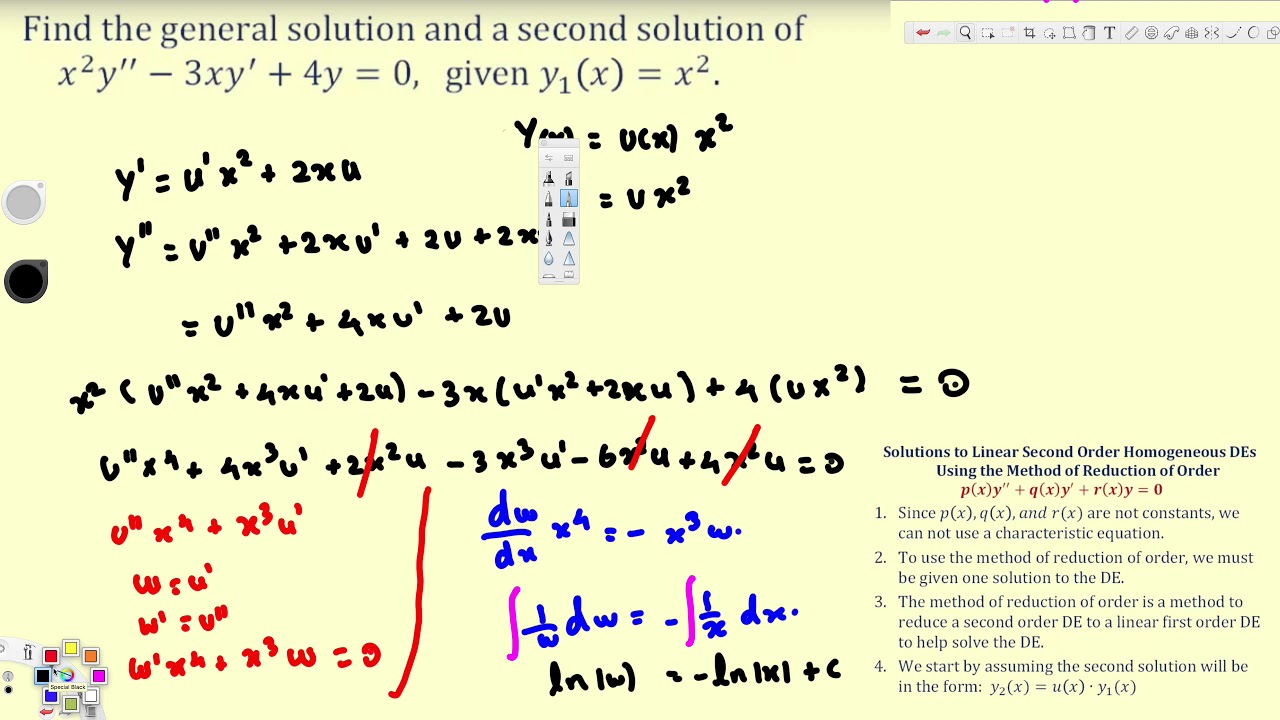
Reduction Of Order Linear Second Order Homogeneous Differential Equations Differential Equations Equations Math

How To Solve Differential Equations Differential Equations Equations Physics And Mathematics

Cauchy Euler Initial Value Problem - Differential Equations In 2021 Differential Equations Equations Initials

Intro To Initial Value Problems 2 Differential Equations Differential Equations Equations Intro

Exact First Order Differential Equations 2 Differential Equations Differential Equations Equations Physics And Mathematics

Solve A First Order Homogeneous Differential Equation 3 - Differential Differential Equations Equations Solving

Exact First Order Differential Equations 1 Differential Equations Differential Equations Equations Math

Verifying Solutions To Differential Equations - Differential Equations 3 Differential Equations Equations Solutions

Solve A First Order Homogeneous Differential Equation 2 - Differential Differential Equations Equations Math

Solve A Bernoulli Differential Equation Initial Value Problem - Differen Differential Equations Physics And Mathematics Equations

Calculus Solving A Differential Equationinitial Value Problem Calculus Differential Equations Maths Exam

Solve A Bernoulli Differential Equation 2 - Differential Equations Differential Equations Equations Solving
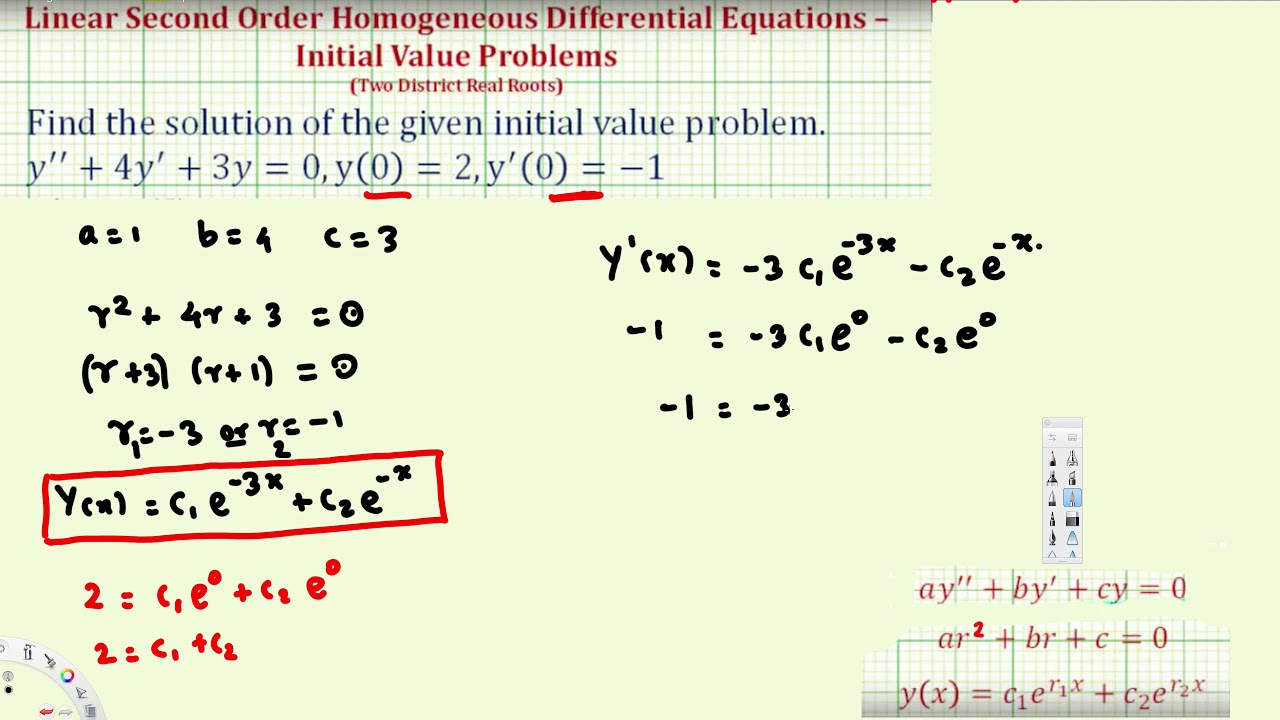
Ex 1 Solve A Linear Second Order Homogeneous Differential Equation Ini Differential Equations Solving Equations

Solve A Linear Second Order Homogeneous Differential Equation Initial Va Differential Equations Solving Equations
Intro To Initial Value Problems 1 - Differential Equations Differential Equations Equations Intro

Intro To Boundary Value Problems - Differential Equations 1 Differential Equations Equations Problem

Ex Solve A Linear Second Order Homogeneous Differential Equation Initi Differential Equations Physics And Mathematics Solving